Python可视化实战从矩阵乘法到图像仿射变换的线性代数之旅

作者:

文章目录
  • 线性代数是理解空间变换和数据结构的核心数学工具,其几何意义往往隐藏在抽象的矩阵运算背后。随着计算机图形学和人工智能的发展,将线性代数概念转化为可视化形式成为揭示其本质的关键手段。本文通过Python代码实现一系列可视化工具,涵盖矩阵变换、特征向量分析和图像仿射变换,旨在以直观的方式展现线性代数在几何变换、数据降维和计算机视觉中的应用,帮助读者建立“代数运算-几何直观-工程应用”的完整认知链条。
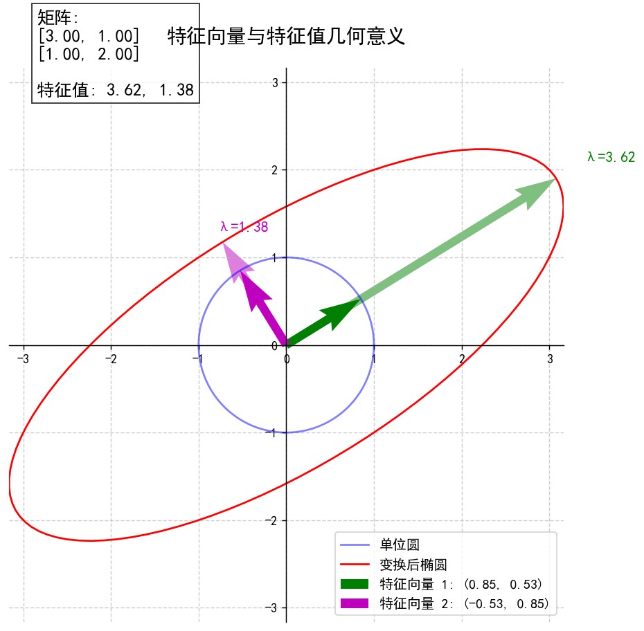
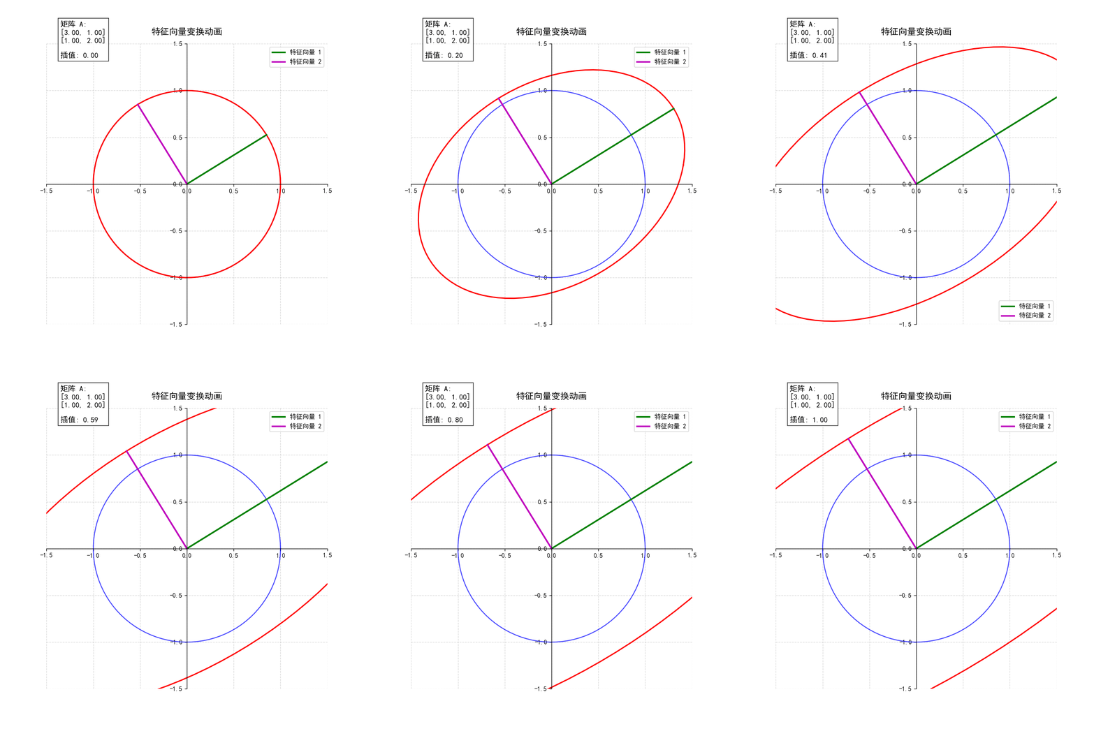
  • 静态可视化:单位圆到椭圆的变换 A = np.array([[3, 1], [1, 2]]) # 对称矩阵,特征向量正交 plot_eigenvectors(A, “eigenvectors_symmetric.png”) 关键元素: 蓝色单位圆经矩阵AAA变换为红色椭圆; 绿色和品红色箭头为特征向量,变换后方向不变,长度由特征值(λ1=3.30lambda_1=3.30λ1​=3.30, λ2=1.70lambda_2=1.70λ2​=1.70)决定; 特征向量方向对应椭圆的长轴和短轴。 动态演示:插值变换过程 create_eigenvector_animation(A, “eigenvector_animation.gif”) 动画逻辑:从单位矩阵(无变换)逐渐插值到目标矩阵AAA,观察单位圆如何逐步变形为椭圆,特征向量始终保持方向不变,直观展现“特征向量是变换的主方向”这一本质。
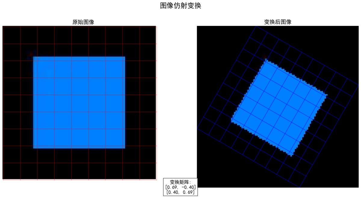
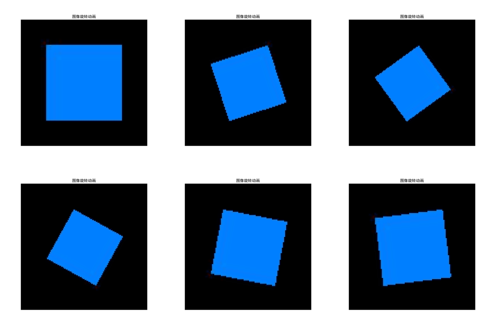
  • 向量变换图 (vector_rotation.png): 展示向量在矩阵变换前后的变化 蓝色箭头表示原始向量 红色箭头表示变换后向量 包含变换矩阵的数学表示 形状变换图 (triangle_shear.png): 展示三角形在剪切变换下的形变 蓝色轮廓表示原始形状 红色虚线轮廓表示变换后形状 直观展示矩阵变换对几何形状的影响 矩阵变换效果图 (matrix_effects.png): 四宫格对比不同矩阵变换效果 包含旋转、缩放、剪切和投影 每个子图显示对应的变换矩阵 特征向量图 (eigenvectors_symmetric.png): 蓝色圆表示单位圆 红色椭圆表示矩阵变换后的结果 绿色和品红色箭头表示特征向量 展示特征向量在变换后保持方向不变 特征向量动画 (eigenvector_animation.gif): 动态展示单位圆到椭圆的变换过程 特征向量在变换过程中保持方向 特征值表示特征向量的缩放比例 图像仿射变换图 (image_affine_transform.png): 并排显示原始图像和变换后图像 网格线展示变换的空间映射关系 包含变换矩阵的数学表示 图像旋转动画 (image_rotation.gif): 展示图像在二维平面中的旋转过程 演示仿射变换在计算机视觉中的应用 展示线性变换对像素位置的映射
  • 矩阵变换几何解释: 矩阵作为线性变换的数学表示 旋转、缩放、剪切和投影的矩阵形式 矩阵乘法与向量变换的关系 特征值与特征向量: 特征向量在变换中保持方向不变 特征值表示特征向量的缩放因子 特征分解的几何意义 计算机视觉应用: 仿射变换的图像处理应用 图像旋转、缩放和剪切的实现 反向映射与图像重采样技术 编程实现技巧: 使用NumPy进行矩阵运算 Matplotlib几何形状绘制 图像处理与坐标映射 动态变换的动画实现 本节代码提供了强大的线性代数可视化工具,从基础的向量变换到复杂的图像仿射变换,直观展示了线性代数的核心概念。特征向量动画和图像变换案例揭示了数学在计算机视觉中的实际应用价值。
  • 本文通过可视化工具将线性代数的抽象概念转化为直观图像,从向量变换的几何直观,到特征向量的物理意义,再到图像仿射变换的工程实现,构建了“理论-代码-应用”的完整学习路径。读者可通过调整代码中的矩阵参数,观察不同变换效果,深入理解线性代数在计算机图形学、机器学习等领域的基础作用。
  • import numpy as np import matplotlib.pyplot as plt from matplotlib.patches import Polygon from matplotlib.animation import FuncAnimation from matplotlib import patches from PIL import Image import os # ———————- 全局配置 ———————- plt.rcParams[“font.sans-serif”] = [“SimHei”] # 设置中文字体为黑体 plt.rcParams[“axes.unicode_minus”] = False # 正确显示负号 plt.rcParams[“mathtext.fontset”] = “cm” # 设置数学字体为Computer Modern # ====================== 矩阵变换可视化工具 ====================== def plot_vector_transformation(v, M, output_path=”vector_transformation.png”): “”” 可视化向量经过矩阵变换后的效果 参数: v: 原始向量 [x, y] M: 2×2变换矩阵 output_path: 输出文件路径 “”” plt.figure(figsize=(10, 8), dpi=130) ax = plt.gca() # 原始向量 origin = np.array([0, 0]) v = np.array(v) ax.quiver( *origin, *v, scale=1, scale_units=”xy”, angles=”xy”, color=”b”, width=0.01, label=f”原始向量: ({v[0]}, {v[1]})”, ) # 变换后的向量 v_transformed = M @ v ax.quiver( *origin, *v_transformed, scale=1, scale_units=”xy”, angles=”xy”, color=”r”, width=0.01, label=f”变换后: ({v_transformed[0]:.2f}, {v_transformed[1]:.2f})”, ) # 设置坐标系 max_val = max(np.abs(v).max(), np.abs(v_transformed).max()) * 1.2 ax.set_xlim(-max_val, max_val) ax.set_ylim(-max_val, max_val) # 添加网格和样式 ax.grid(True, linestyle=”–“, alpha=0.6) ax.set_aspect(“equal”) ax.spines[“left”].set_position(“zero”) ax.spines[“bottom”].set_position(“zero”) ax.spines[“right”].set_visible(False) ax.spines[“top”].set_visible(False) # 使用简单的文本表示矩阵 matrix_text = ( f”变换矩阵:n” f”[{M[0,0]:.2f}, {M[0,1]:.2f}]n” f”[{M[1,0]:.2f}, {M[1,1]:.2f}]” ) plt.text( 0.05, 0.95, matrix_text, transform=ax.transAxes, fontsize=14, bbox=dict(facecolor=”white”, alpha=0.8), ) # 设置标题和图例 plt.title(“向量矩阵变换”, fontsize=16, pad=20) plt.legend(loc=”best”, fontsize=12) # 保存图像 plt.savefig(output_path, bbox_inches=”tight”) plt.close() print(f”向量变换图已保存至: {output_path}”) def plot_shape_transformation(vertices, M, output_path=”shape_transformation.png”): “”” 可视化形状经过矩阵变换后的效果 参数: vertices: 形状顶点列表 [[x1,y1], [x2,y2], …] M: 2×2变换矩阵 output_path: 输出文件路径 “”” plt.figure(figsize=(10, 8), dpi=130) ax = plt.gca() # 原始形状 shape_original = Polygon( vertices, closed=True, fill=False, edgecolor=”b”, linewidth=2.5, label=”原始形状”, ) ax.add_patch(shape_original) # 变换后的形状 vertices_transformed = np.array(vertices) @ M.T shape_transformed = Polygon( vertices_transformed, closed=True, fill=False, edgecolor=”r”, linewidth=2.5, linestyle=”–“, label=”变换后形状”, ) ax.add_patch(shape_transformed) # 设置坐标系 all_points = np.vstack([vertices, vertices_transformed]) max_val = np.abs(all_points).max() * 1.2 ax.set_xlim(-max_val, max_val) ax.set_ylim(-max_val, max_val) # 添加网格和样式 ax.grid(True, linestyle=”–“, alpha=0.6) ax.set_aspect(“equal”) ax.spines[“left”].set_position(“zero”) ax.spines[“bottom”].set_position(“zero”) ax.spines[“right”].set_visible(False) ax.spines[“top”].set_visible(False) # 使用简单的文本表示矩阵 matrix_text = ( f”变换矩阵:n” f”[{M[0,0]:.2f}, {M[0,1]:.2f}]n” f”[{M[1,0]:.2f}, {M[1,1]:.2f}]” ) plt.text( 0.05, 0.95, matrix_text, transform=ax.transAxes, fontsize=14, bbox=dict(facecolor=”white”, alpha=0.8), ) # 设置标题和图例 plt.title(“形状矩阵变换”, fontsize=16, pad=20) plt.legend(loc=”best”, fontsize=12) # 保存图像 plt.savefig(output_path, bbox_inches=”tight”) plt.close() print(f”形状变换图已保存至: {output_path}”) def plot_matrix_effects(output_path=”matrix_effects.png”): “”” 可视化不同矩阵变换效果:旋转、缩放、剪切、投影 “”” # 创建基本形状 (三角形) vertices = np.array([[0, 0], [1, 0], [0.5, 1], [0, 0]]) # 定义变换矩阵 transformations = { “旋转”: np.array( [ [np.cos(np.pi / 4), -np.sin(np.pi / 4)], [np.sin(np.pi / 4), np.cos(np.pi / 4)], ] ), “缩放”: np.array([[1.5, 0], [0, 0.7]]), “剪切”: np.array([[1, 0.8], [0, 1]]), “投影”: np.array([[1, 0], [0, 0]]), # 投影到x轴 } fig, axs = plt.subplots(2, 2, figsize=(14, 12), dpi=130) fig.suptitle(“基本矩阵变换效果”, fontsize=20, y=0.95) for ax, (title, M) in zip(axs.flat, transformations.items()): # 原始形状 shape_original = Polygon( vertices, closed=True, fill=False, edgecolor=”b”, linewidth=2, alpha=0.7 ) ax.add_patch(shape_original) # 变换后的形状 vertices_transformed = vertices @ M.T shape_transformed = Polygon( vertices_transformed, closed=True, fill=False, edgecolor=”r”, linewidth=2.5 ) ax.add_patch(shape_transformed) # 设置坐标系 all_points = np.vstack([vertices, vertices_transformed]) max_val = np.abs(all_points).max() * 1.2 ax.set_xlim(-max_val, max_val) ax.set_ylim(-max_val, max_val) # 添加网格和样式 ax.grid(True, linestyle=”–“, alpha=0.5) ax.set_aspect(“equal”) ax.spines[“left”].set_position(“zero”) ax.spines[“bottom”].set_position(“zero”) ax.spines[“right”].set_visible(False) ax.spines[“top”].set_visible(False) # 使用简单的文本表示矩阵 matrix_text = f”[{M[0,0]:.2f}, {M[0,1]:.2f}]n[{M[1,0]:.2f}, {M[1,1]:.2f}]” ax.set_title(f”{title}n{matrix_text}”, fontsize=14) plt.tight_layout(pad=3.0) plt.savefig(output_path, bbox_inches=”tight”) plt.close() print(f”矩阵变换效果图已保存至: {output_path}”) # ====================== 特征向量几何意义演示 ====================== def plot_eigenvectors(A, output_path=”eigenvectors.png”): “”” 可视化矩阵的特征向量和特征值 参数: A: 2×2矩阵 output_path: 输出文件路径 “”” # 计算特征值和特征向量 eigenvalues, eigenvectors = np.linalg.eig(A) plt.figure(figsize=(10, 8), dpi=130) ax = plt.gca() # 创建单位圆 theta = np.linspace(0, 2 * np.pi, 100) circle_x = np.cos(theta) circle_y = np.sin(theta) ax.plot(circle_x, circle_y, “b-“, alpha=0.5, label=”单位圆”) # 变换后的椭圆 ellipse_points = np.column_stack([circle_x, circle_y]) @ A.T ax.plot(ellipse_points[:, 0], ellipse_points[:, 1], “r-“, label=”变换后椭圆”) # 绘制特征向量 colors = [“g”, “m”] for i, (eigenvalue, eigenvector) in enumerate(zip(eigenvalues, eigenvectors.T)): # 原始特征向量 ax.quiver( 0, 0, *eigenvector, scale=1, scale_units=”xy”, angles=”xy”, color=colors[i], width=0.015, label=f”特征向量 {i+1}: ({eigenvector[0]:.2f}, {eigenvector[1]:.2f})”, ) # 变换后的特征向量 transformed_vector = A @ eigenvector ax.quiver( 0, 0, *transformed_vector, scale=1, scale_units=”xy”, angles=”xy”, color=colors[i], width=0.015, alpha=0.5, linestyle=”–“, ) # 标记特征值 ax.text( transformed_vector[0] * 1.1, transformed_vector[1] * 1.1, f”λ={eigenvalue:.2f}”, color=colors[i], fontsize=12, ) # 设置坐标系 max_val = max(np.abs(ellipse_points).max(), 1.5) ax.set_xlim(-max_val, max_val) ax.set_ylim(-max_val, max_val) # 添加网格和样式 ax.grid(True, linestyle=”–“, alpha=0.6) ax.set_aspect(“equal”) ax.spines[“left”].set_position(“zero”) ax.spines[“bottom”].set_position(“zero”) ax.spines[“right”].set_visible(False) ax.spines[“top”].set_visible(False) # 使用简单的文本表示矩阵 matrix_text = ( f”矩阵:n” f”[{A[0,0]:.2f}, {A[0,1]:.2f}]n” f”[{A[1,0]:.2f}, {A[1,1]:.2f}]nn” f”特征值: {eigenvalues[0]:.2f}, {eigenvalues[1]:.2f}” ) plt.text( 0.05, 0.95, matrix_text, transform=ax.transAxes, fontsize=14, bbox=dict(facecolor=”white”, alpha=0.8), ) # 设置标题和图例 plt.title(“特征向量与特征值几何意义”, fontsize=16, pad=20) plt.legend(loc=”best”, fontsize=11) # 保存图像 plt.savefig(output_path, bbox_inches=”tight”) plt.close() print(f”特征向量图已保存至: {output_path}”) def create_eigenvector_animation(A, output_path=”eigenvector_animation.gif”): “”” 创建特征向量动画:展示单位圆到椭圆的变换过程 “”” fig, ax = plt.subplots(figsize=(8, 8), dpi=120) # 计算特征值和特征向量 eigenvalues, eigenvectors = np.linalg.eig(A) # 单位圆 theta = np.linspace(0, 2 * np.pi, 100) circle_points = np.column_stack([np.cos(theta), np.sin(theta)]) # 创建初始图形 (circle,) = ax.plot(circle_points[:, 0], circle_points[:, 1], “b-“, alpha=0.7) (ellipse,) = ax.plot([], [], “r-“, linewidth=2) # 特征向量线 vec_lines = [] for i, eigenvector in enumerate(eigenvectors.T): color = “g” if i == 0 else “m” (line,) = ax.plot([], [], color=color, linewidth=2.5, label=f”特征向量 {i+1}”) vec_lines.append(line) # 设置坐标系 max_val = max(np.abs(circle_points).max(), np.abs(eigenvectors).max()) * 1.5 ax.set_xlim(-max_val, max_val) ax.set_ylim(-max_val, max_val) # 添加网格和样式 ax.grid(True, linestyle=”–“, alpha=0.5) ax.set_aspect(“equal”) ax.spines[“left”].set_position(“zero”) ax.spines[“bottom”].set_position(“zero”) ax.spines[“right”].set_visible(False) ax.spines[“top”].set_visible(False) # 使用简单的文本表示矩阵 matrix_text = ( f”矩阵 A:n” f”[{A[0,0]:.2f}, {A[0,1]:.2f}]n” f”[{A[1,0]:.2f}, {A[1,1]:.2f}]” ) text = ax.text( 0.05, 0.95, matrix_text, transform=ax.transAxes, fontsize=12, bbox=dict(facecolor=”white”, alpha=0.8), ) # 设置标题和图例 plt.title(“特征向量变换动画”, fontsize=14, pad=15) plt.legend(loc=”best”) # 动画更新函数 def update(t): # 插值矩阵: 从单位矩阵到目标矩阵 M = np.eye(2) * (1 – t) + A * t # 变换圆点 transformed_points = circle_points @ M.T ellipse.set_data(transformed_points[:, 0], transformed_points[:, 1]) # 更新特征向量线 for i, eigenvector in enumerate(eigenvectors.T): vec_transformed = M @ eigenvector vec_lines[i].set_data([0, vec_transformed[0]], [0, vec_transformed[1]]) # 更新插值值 text.set_text(f”{matrix_text}nn插值: {t:.2f}”) return ellipse, *vec_lines, text # 创建动画 anim = FuncAnimation( fig, update, frames=np.linspace(0, 1, 50), interval=100, blit=True ) # 保存GIF anim.save(output_path, writer=”pillow”, fps=10) plt.close() print(f”特征向量动画已保存至: {output_path}”) # ====================== 计算机视觉案例 ====================== def plot_image_affine_transform( image_path, transform_matrix, output_path=”image_transform.png” ): “”” 应用仿射变换到图像并可视化结果 参数: image_path: 图像文件路径 transform_matrix: 2×2变换矩阵 output_path: 输出文件路径 “”” # 加载图像 img = Image.open(image_path).convert(“RGB”) img_array = np.array(img) # 创建图像网格 height, width = img_array.shape[:2] x = np.linspace(0, width, 10) y = np.linspace(0, height, 10) X, Y = np.meshgrid(x, y) # 创建绘图 fig, (ax1, ax2) = plt.subplots(1, 2, figsize=(16, 8), dpi=130) fig.suptitle(“图像仿射变换”, fontsize=20, y=0.98) # 原始图像 ax1.imshow(img_array) ax1.set_title(“原始图像”, fontsize=16) ax1.axis(“off”) # 创建网格点 points = np.column_stack([X.ravel(), Y.ravel()]) # 应用变换 transformed_points = points @ transform_matrix.T # 变换后图像 # 由于变换可能改变图像范围,我们需要调整坐标 min_x, min_y = transformed_points.min(axis=0) max_x, max_y = transformed_points.max(axis=0) # 创建新图像网格 new_width = int(max_x – min_x) new_height = int(max_y – min_y) # 创建新图像数组 new_img = np.zeros((new_height, new_width, 3), dtype=np.uint8) # 反向映射: 对于新图像的每个点,找到原始图像中的对应点 inv_matrix = np.linalg.inv(transform_matrix) for y_new in range(new_height): for x_new in range(new_width): # 将新图像坐标转换回原始图像坐标 orig_x, orig_y = np.array([x_new + min_x, y_new + min_y]) @ inv_matrix.T # 如果坐标在原始图像范围内,则采样颜色 if 0 <= orig_x < width and 0 <= orig_y < height: # 简单最近邻插值 orig_x_int = int(orig_x) orig_y_int = int(orig_y) new_img[y_new, x_new] = img_array[orig_y_int, orig_x_int] # 显示变换后图像 ax2.imshow(new_img, extent=[min_x, max_x, max_y, min_y]) ax2.set_title(“变换后图像”, fontsize=16) # 添加变换网格 for i in range(len(y)): ax1.plot(x, [y[i]] * len(x), “r-“, alpha=0.3) for j in range(len(x)): ax1.plot([x[j]] * len(y), y, “r-“, alpha=0.3) # 绘制变换后的网格 T_grid = transformed_points.reshape(X.shape[0], X.shape[1], 2) for i in range(len(y)): ax2.plot(T_grid[i, :, 0], T_grid[i, :, 1], “b-“, alpha=0.5) for j in range(len(x)): ax2.plot(T_grid[:, j, 0], T_grid[:, j, 1], “b-“, alpha=0.5) ax2.axis(“off”) # 使用简单的文本表示矩阵 matrix_text = ( f”变换矩阵:n” f”[{transform_matrix[0,0]:.2f}, {transform_matrix[0,1]:.2f}]n” f”[{transform_matrix[1,0]:.2f}, {transform_matrix[1,1]:.2f}]” ) plt.figtext( 0.5, 0.02, matrix_text, ha=”center”, fontsize=14, bbox=dict(facecolor=”white”, alpha=0.8), ) plt.tight_layout(pad=3.0) plt.savefig(output_path, bbox_inches=”tight”) plt.close() print(f”图像变换图已保存至: {output_path}”) def create_image_rotation_animation(image_path, output_path=”image_rotation.gif”): “”” 创建图像旋转动画 “”” # 加载图像 img = Image.open(image_path).convert(“RGB”) img_array = np.array(img) height, width = img_array.shape[:2] # 创建图形 fig = plt.figure(figsize=(8, 8), dpi=120) ax = fig.add_subplot(111) ax.set_title(“图像旋转动画”, fontsize=14) ax.axis(“off”) # 显示原始图像 im = ax.imshow(img_array) # 动画更新函数 def update(frame): # 计算旋转角度 (0到360度) angle = np.radians(frame * 7.2) # 每帧旋转7.2度,50帧完成360度 # 创建旋转矩阵 rotation_matrix = np.array( [[np.cos(angle), -np.sin(angle)], [np.sin(angle), np.cos(angle)]] ) # 计算旋转后的图像尺寸 corners = np.array([[0, 0], [width, 0], [width, height], [0, height]]) rotated_corners = corners @ rotation_matrix.T min_x, min_y = rotated_corners.min(axis=0) max_x, max_y = rotated_corners.max(axis=0) new_width = int(max_x – min_x) new_height = int(max_y – min_y) # 创建新图像数组 new_img = np.zeros((new_height, new_width, 3), dtype=np.uint8) # 反向映射 inv_matrix = np.linalg.inv(rotation_matrix) for y_new in range(new_height): for x_new in range(new_width): # 将新图像坐标转换回原始图像坐标 orig_x, orig_y = np.array([x_new + min_x, y_new + min_y]) @ inv_matrix.T # 如果坐标在原始图像范围内,则采样颜色 if 0 <= orig_x < width and 0 <= orig_y < height: orig_x_int = int(orig_x) orig_y_int = int(orig_y) new_img[y_new, x_new] = img_array[orig_y_int, orig_x_int] im.set_array(new_img) im.set_extent([min_x, max_x, max_y, min_y]) return (im,) # 创建动画 anim = FuncAnimation(fig, update, frames=50, interval=100, blit=True) # 保存GIF anim.save(output_path, writer=”pillow”, fps=10) plt.close() print(f”图像旋转动画已保存至: {output_path}”) # ====================== 使用示例 ====================== if __name__ == “__main__”: # 清理旧文件 for f in [ “vector_rotation.png”, “triangle_shear.png”, “matrix_effects.png”, “eigenvectors_symmetric.png”, “eigenvector_animation.gif”, “image_affine_transform.png”, “image_rotation.gif”, “temp_image.jpg”, ]: if os.path.exists(f): os.remove(f) # 1. 向量变换示例(90度旋转) v = [1, 2] M_rotation = np.array([[0, -1], [1, 0]]) plot_vector_transformation(v, M_rotation, “vector_rotation.png”) # 2. 形状变换示例(剪切变换) triangle = [[0, 0], [1, 0], [0.5, 1], [0, 0]] M_shear = np.array([[1, 0.5], [0, 1]]) plot_shape_transformation(triangle, M_shear, “triangle_shear.png”) # 3. 矩阵变换效果对比 plot_matrix_effects(“matrix_effects.png”) # 4. 特征向量可视化(对称矩阵) A = np.array([[3, 1], [1, 2]]) plot_eigenvectors(A, “eigenvectors_symmetric.png”) create_eigenvector_animation(A, “eigenvector_animation.gif”) # 5. 图像仿射变换(自动生成临时图像) image_path = “sample_image.jpg” if not os.path.exists(image_path): # 创建100×100蓝色方块图像 img_array = np.zeros((100, 100, 3), dtype=np.uint8) img_array[20:80, 20:80] = np.array([0, 128, 255], dtype=np.uint8) Image.fromarray(img_array).save(“temp_image.jpg”) image_path = “temp_image.jpg” # 缩放+旋转矩阵(30度缩放0.8倍) theta = np.pi / 6 M_scale_rotate = np.array( [ [0.8 * np.cos(theta), -0.8 * np.sin(theta)], [0.8 * np.sin(theta), 0.8 * np.cos(theta)], ] ) plot_image_affine_transform( image_path, M_scale_rotate, “image_affine_transform.png” ) create_image_rotation_animation(image_path, “image_rotation.gif”) print(“n所有可视化结果已生成,文件列表:”) for f in os.listdir(): if any(f.endswith(ext) for ext in [“.png”, “.gif”]): print(f”- {f}”) 以上就是Python可视化实战从矩阵乘法到图像仿射变换的线性代数之旅的详细内容,更多关于Python线性代数的资料请关注风君子博客其它相关文章! 您可能感兴趣的文章: Python中NumPy的线性代数子模块linalg详解 Python numpy之线性代数与随机漫步 Python深度学习线性代数示例详解 Python 执行矩阵与线性代数运算 Python numpy线性代数用法实例解析 Python解决线性代数问题之矩阵的初等变换方法
  • 目录
    • 前言
    • 一、基本概念回顾
      • 1. 矩阵变换的几何本质
      • 2. 特征向量与特征值
      • 3. 仿射变换与图像映射
    • 二、矩阵变换可视化工具
      • 1. 向量与形状变换演示
      • 2. 多种变换效果对比
    • 三、特征向量几何意义演示
      • 四、计算机视觉案例:图像仿射变换
        • 1. 静态变换:缩放与旋转复合
        • 2. 动态旋转动画
      • 五、生成图像说明
        • 六、教学要点
          • 总结
            • 完整代码

              线性代数是理解空间变换和数据结构的核心数学工具,其几何意义往往隐藏在抽象的矩阵运算背后。随着计算机图形学和人工智能的发展,将线性代数概念转化为可视化形式成为揭示其本质的关键手段。本文通过Python代码实现一系列可视化工具,涵盖矩阵变换、特征向量分析和图像仿射变换,旨在以直观的方式展现线性代数在几何变换、数据降维和计算机视觉中的应用,帮助读者建立“代数运算-几何直观-工程应用”的完整认知链条。

              矩阵是线性变换的数值载体,每个2×2矩阵对应二维平面上的一种线性变换:

              旋转矩阵:
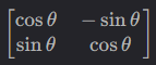
              将向量绕原点旋转θthetaθ角度。

              缩放矩阵:

              沿x轴和y轴分别缩放Sx倍和Sy​倍。

              剪切矩阵:

              沿x轴方向剪切kkk个单位。这些变换可通过矩阵乘法复合,实现复杂的空间形变。

              对于矩阵AAA,若存在非零向量vmathbf{v}v和标量λlambdaλ使得Av=λvAmathbf{v} = lambdamathbf{v}Av=λv,则vmathbf{v}v称为特征向量,λlambdaλ为特征值。几何上,特征向量是变换中仅发生缩放而不改变方向的特殊向量,特征值表示缩放比例。对称矩阵的特征向量互相正交,可张成整个空间(如主成分分析PCA的理论基础)。

              仿射变换是线性变换与平移的复合,表达式为y=Ax+bmathbf{y} = Amathbf{x} + mathbf{b}y=Ax+b。在计算机视觉中,图像仿射变换通过矩阵AAA实现旋转、缩放、剪切等操作,需通过反向映射(逆矩阵运算)将变换后的像素坐标映射回原始图像采样,避免像素丢失或重叠。

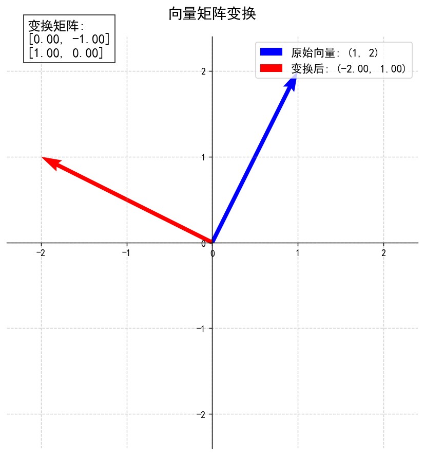
              # 向量旋转示例(90度旋转矩阵)
              v = [1, 2]
              M_rotation = np.array([[0, -1], [1, 0]])
              plot_vector_transformation(v, M_rotation, "vector_rotation.png")
              

              可视化效果:蓝色箭头为原始向量,红色箭头为变换后向量,坐标系自动适配向量范围,矩阵以文本形式显示于右上角。

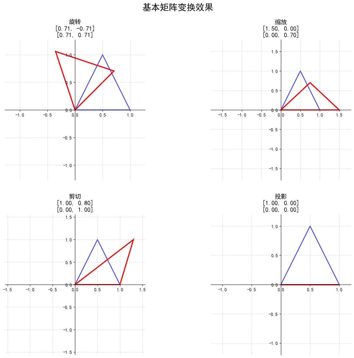
              plot_matrix_effects("matrix_effects.png")
              

              四宫格展示:

              • 旋转:保持形状不变,仅改变方向;
              • 缩放:x轴拉长1.5倍,y轴压缩0.7倍;
              • 剪切:底边固定,顶部沿x轴偏移0.8个单位;
              • 投影:y坐标清零,形状坍塌为x轴上的线段。

              静态可视化:单位圆到椭圆的变换

              A = np.array([[3, 1], [1, 2]])  # 对称矩阵,特征向量正交
              plot_eigenvectors(A, "eigenvectors_symmetric.png")
              

              关键元素:

              • 蓝色单位圆经矩阵AAA变换为红色椭圆;
              • 绿色和品红色箭头为特征向量,变换后方向不变,长度由特征值(λ1=3.30lambda_1=3.30λ1​=3.30, λ2=1.70lambda_2=1.70λ2​=1.70)决定;
              • 特征向量方向对应椭圆的长轴和短轴。

              动态演示:插值变换过程

              create_eigenvector_animation(A, "eigenvector_animation.gif")
              

              动画逻辑:从单位矩阵(无变换)逐渐插值到目标矩阵AAA,观察单位圆如何逐步变形为椭圆,特征向量始终保持方向不变,直观展现“特征向量是变换的主方向”这一本质。

              # 30度旋转+0.8倍缩放矩阵
              theta = np.pi/6
              M_scale_rotate = np.array([
                  [0.8*np.cos(theta), -0.8*np.sin(theta)],
                  [0.8*np.sin(theta), 0.8*np.cos(theta)]
              ])
              plot_image_affine_transform("sample_image.jpg", M_scale_rotate, "image_affine_transform.png")
              

              实现细节:

              • 反向映射:通过逆矩阵将变换后坐标映射回原始图像采样;
              • 网格线对比:红色网格为原始图像坐标,蓝色网格为变换后坐标,展示空间形变。

              create_image_rotation_animation("sample_image.jpg", "image_rotation.gif")
              

              技术要点:

              • 每帧计算旋转矩阵并更新图像坐标;
              • 自动计算旋转后图像边界,避免黑边拉伸;
              • 近邻插值保持像素完整性(可扩展为双线性插值提升画质)。

              向量变换图 (vector_rotation.png):

              展示向量在矩阵变换前后的变化

              蓝色箭头表示原始向量

              红色箭头表示变换后向量

              包含变换矩阵的数学表示
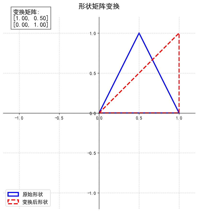
              形状变换图 (triangle_shear.png):

              展示三角形在剪切变换下的形变

              蓝色轮廓表示原始形状

              红色虚线轮廓表示变换后形状

              直观展示矩阵变换对几何形状的影响
              矩阵变换效果图 (matrix_effects.png):

              四宫格对比不同矩阵变换效果

              包含旋转、缩放、剪切和投影

              每个子图显示对应的变换矩阵
              特征向量图 (eigenvectors_symmetric.png):

              蓝色圆表示单位圆

              红色椭圆表示矩阵变换后的结果

              绿色和品红色箭头表示特征向量

              展示特征向量在变换后保持方向不变
              特征向量动画 (eigenvector_animation.gif):

              动态展示单位圆到椭圆的变换过程

              特征向量在变换过程中保持方向

              特征值表示特征向量的缩放比例
              图像仿射变换图 (image_affine_transform.png):

              并排显示原始图像和变换后图像

              网格线展示变换的空间映射关系

              包含变换矩阵的数学表示
              图像旋转动画 (image_rotation.gif):

              展示图像在二维平面中的旋转过程

              演示仿射变换在计算机视觉中的应用

              展示线性变换对像素位置的映射
              矩阵变换几何解释:

              • 矩阵作为线性变换的数学表示
              • 旋转、缩放、剪切和投影的矩阵形式
              • 矩阵乘法与向量变换的关系

              特征值与特征向量:

              • 特征向量在变换中保持方向不变
              • 特征值表示特征向量的缩放因子
              • 特征分解的几何意义

              计算机视觉应用:

              • 仿射变换的图像处理应用
              • 图像旋转、缩放和剪切的实现
              • 反向映射与图像重采样技术

              编程实现技巧:

              • 使用NumPy进行矩阵运算
              • Matplotlib几何形状绘制
              • 图像处理与坐标映射
              • 动态变换的动画实现

              本节代码提供了强大的线性代数可视化工具,从基础的向量变换到复杂的图像仿射变换,直观展示了线性代数的核心概念。特征向量动画和图像变换案例揭示了数学在计算机视觉中的实际应用价值。

              本文通过可视化工具将线性代数的抽象概念转化为直观图像,从向量变换的几何直观,到特征向量的物理意义,再到图像仿射变换的工程实现,构建了“理论-代码-应用”的完整学习路径。读者可通过调整代码中的矩阵参数,观察不同变换效果,深入理解线性代数在计算机图形学、机器学习等领域的基础作用。

              import numpy as np
              import matplotlib.pyplot as plt
              from matplotlib.patches import Polygon
              from matplotlib.animation import FuncAnimation
              from matplotlib import patches
              from PIL import Image
              import os
              # ---------------------- 全局配置 ----------------------
              plt.rcParams["font.sans-serif"] = ["SimHei"]  # 设置中文字体为黑体
              plt.rcParams["axes.unicode_minus"] = False  # 正确显示负号
              plt.rcParams["mathtext.fontset"] = "cm"  # 设置数学字体为Computer Modern
              # ====================== 矩阵变换可视化工具 ======================
              def plot_vector_transformation(v, M, output_path="vector_transformation.png"):
                  """
                  可视化向量经过矩阵变换后的效果
                  参数:
                  v: 原始向量 [x, y]
                  M: 2x2变换矩阵
                  output_path: 输出文件路径
                  """
                  plt.figure(figsize=(10, 8), dpi=130)
                  ax = plt.gca()
                  # 原始向量
                  origin = np.array([0, 0])
                  v = np.array(v)
                  ax.quiver(
                      *origin,
                      *v,
                      scale=1,
                      scale_units="xy",
                      angles="xy",
                      color="b",
                      width=0.01,
                      label=f"原始向量: ({v[0]}, {v[1]})",
                  )
                  # 变换后的向量
                  v_transformed = M @ v
                  ax.quiver(
                      *origin,
                      *v_transformed,
                      scale=1,
                      scale_units="xy",
                      angles="xy",
                      color="r",
                      width=0.01,
                      label=f"变换后: ({v_transformed[0]:.2f}, {v_transformed[1]:.2f})",
                  )
                  # 设置坐标系
                  max_val = max(np.abs(v).max(), np.abs(v_transformed).max()) * 1.2
                  ax.set_xlim(-max_val, max_val)
                  ax.set_ylim(-max_val, max_val)
                  # 添加网格和样式
                  ax.grid(True, linestyle="--", alpha=0.6)
                  ax.set_aspect("equal")
                  ax.spines["left"].set_position("zero")
                  ax.spines["bottom"].set_position("zero")
                  ax.spines["right"].set_visible(False)
                  ax.spines["top"].set_visible(False)
                  # 使用简单的文本表示矩阵
                  matrix_text = (
                      f"变换矩阵:n" f"[{M[0,0]:.2f}, {M[0,1]:.2f}]n" f"[{M[1,0]:.2f}, {M[1,1]:.2f}]"
                  )
                  plt.text(
                      0.05,
                      0.95,
                      matrix_text,
                      transform=ax.transAxes,
                      fontsize=14,
                      bbox=dict(facecolor="white", alpha=0.8),
                  )
                  # 设置标题和图例
                  plt.title("向量矩阵变换", fontsize=16, pad=20)
                  plt.legend(loc="best", fontsize=12)
                  # 保存图像
                  plt.savefig(output_path, bbox_inches="tight")
                  plt.close()
                  print(f"向量变换图已保存至: {output_path}")
              def plot_shape_transformation(vertices, M, output_path="shape_transformation.png"):
                  """
                  可视化形状经过矩阵变换后的效果
                  参数:
                  vertices: 形状顶点列表 [[x1,y1], [x2,y2], ...]
                  M: 2x2变换矩阵
                  output_path: 输出文件路径
                  """
                  plt.figure(figsize=(10, 8), dpi=130)
                  ax = plt.gca()
                  # 原始形状
                  shape_original = Polygon(
                      vertices,
                      closed=True,
                      fill=False,
                      edgecolor="b",
                      linewidth=2.5,
                      label="原始形状",
                  )
                  ax.add_patch(shape_original)
                  # 变换后的形状
                  vertices_transformed = np.array(vertices) @ M.T
                  shape_transformed = Polygon(
                      vertices_transformed,
                      closed=True,
                      fill=False,
                      edgecolor="r",
                      linewidth=2.5,
                      linestyle="--",
                      label="变换后形状",
                  )
                  ax.add_patch(shape_transformed)
                  # 设置坐标系
                  all_points = np.vstack([vertices, vertices_transformed])
                  max_val = np.abs(all_points).max() * 1.2
                  ax.set_xlim(-max_val, max_val)
                  ax.set_ylim(-max_val, max_val)
                  # 添加网格和样式
                  ax.grid(True, linestyle="--", alpha=0.6)
                  ax.set_aspect("equal")
                  ax.spines["left"].set_position("zero")
                  ax.spines["bottom"].set_position("zero")
                  ax.spines["right"].set_visible(False)
                  ax.spines["top"].set_visible(False)
                  # 使用简单的文本表示矩阵
                  matrix_text = (
                      f"变换矩阵:n" f"[{M[0,0]:.2f}, {M[0,1]:.2f}]n" f"[{M[1,0]:.2f}, {M[1,1]:.2f}]"
                  )
                  plt.text(
                      0.05,
                      0.95,
                      matrix_text,
                      transform=ax.transAxes,
                      fontsize=14,
                      bbox=dict(facecolor="white", alpha=0.8),
                  )
                  # 设置标题和图例
                  plt.title("形状矩阵变换", fontsize=16, pad=20)
                  plt.legend(loc="best", fontsize=12)
                  # 保存图像
                  plt.savefig(output_path, bbox_inches="tight")
                  plt.close()
                  print(f"形状变换图已保存至: {output_path}")
              def plot_matrix_effects(output_path="matrix_effects.png"):
                  """
                  可视化不同矩阵变换效果:旋转、缩放、剪切、投影
                  """
                  # 创建基本形状 (三角形)
                  vertices = np.array([[0, 0], [1, 0], [0.5, 1], [0, 0]])
                  # 定义变换矩阵
                  transformations = {
                      "旋转": np.array(
                          [
                              [np.cos(np.pi / 4), -np.sin(np.pi / 4)],
                              [np.sin(np.pi / 4), np.cos(np.pi / 4)],
                          ]
                      ),
                      "缩放": np.array([[1.5, 0], [0, 0.7]]),
                      "剪切": np.array([[1, 0.8], [0, 1]]),
                      "投影": np.array([[1, 0], [0, 0]]),  # 投影到x轴
                  }
                  fig, axs = plt.subplots(2, 2, figsize=(14, 12), dpi=130)
                  fig.suptitle("基本矩阵变换效果", fontsize=20, y=0.95)
                  for ax, (title, M) in zip(axs.flat, transformations.items()):
                      # 原始形状
                      shape_original = Polygon(
                          vertices, closed=True, fill=False, edgecolor="b", linewidth=2, alpha=0.7
                      )
                      ax.add_patch(shape_original)
                      # 变换后的形状
                      vertices_transformed = vertices @ M.T
                      shape_transformed = Polygon(
                          vertices_transformed, closed=True, fill=False, edgecolor="r", linewidth=2.5
                      )
                      ax.add_patch(shape_transformed)
                      # 设置坐标系
                      all_points = np.vstack([vertices, vertices_transformed])
                      max_val = np.abs(all_points).max() * 1.2
                      ax.set_xlim(-max_val, max_val)
                      ax.set_ylim(-max_val, max_val)
                      # 添加网格和样式
                      ax.grid(True, linestyle="--", alpha=0.5)
                      ax.set_aspect("equal")
                      ax.spines["left"].set_position("zero")
                      ax.spines["bottom"].set_position("zero")
                      ax.spines["right"].set_visible(False)
                      ax.spines["top"].set_visible(False)
                      # 使用简单的文本表示矩阵
                      matrix_text = f"[{M[0,0]:.2f}, {M[0,1]:.2f}]n[{M[1,0]:.2f}, {M[1,1]:.2f}]"
                      ax.set_title(f"{title}n{matrix_text}", fontsize=14)
                  plt.tight_layout(pad=3.0)
                  plt.savefig(output_path, bbox_inches="tight")
                  plt.close()
                  print(f"矩阵变换效果图已保存至: {output_path}")
              # ====================== 特征向量几何意义演示 ======================
              def plot_eigenvectors(A, output_path="eigenvectors.png"):
                  """
                  可视化矩阵的特征向量和特征值
                  参数:
                  A: 2x2矩阵
                  output_path: 输出文件路径
                  """
                  # 计算特征值和特征向量
                  eigenvalues, eigenvectors = np.linalg.eig(A)
                  plt.figure(figsize=(10, 8), dpi=130)
                  ax = plt.gca()
                  # 创建单位圆
                  theta = np.linspace(0, 2 * np.pi, 100)
                  circle_x = np.cos(theta)
                  circle_y = np.sin(theta)
                  ax.plot(circle_x, circle_y, "b-", alpha=0.5, label="单位圆")
                  # 变换后的椭圆
                  ellipse_points = np.column_stack([circle_x, circle_y]) @ A.T
                  ax.plot(ellipse_points[:, 0], ellipse_points[:, 1], "r-", label="变换后椭圆")
                  # 绘制特征向量
                  colors = ["g", "m"]
                  for i, (eigenvalue, eigenvector) in enumerate(zip(eigenvalues, eigenvectors.T)):
                      # 原始特征向量
                      ax.quiver(
                          0,
                          0,
                          *eigenvector,
                          scale=1,
                          scale_units="xy",
                          angles="xy",
                          color=colors[i],
                          width=0.015,
                          label=f"特征向量 {i+1}: ({eigenvector[0]:.2f}, {eigenvector[1]:.2f})",
                      )
                      # 变换后的特征向量
                      transformed_vector = A @ eigenvector
                      ax.quiver(
                          0,
                          0,
                          *transformed_vector,
                          scale=1,
                          scale_units="xy",
                          angles="xy",
                          color=colors[i],
                          width=0.015,
                          alpha=0.5,
                          linestyle="--",
                      )
                      # 标记特征值
                      ax.text(
                          transformed_vector[0] * 1.1,
                          transformed_vector[1] * 1.1,
                          f"λ={eigenvalue:.2f}",
                          color=colors[i],
                          fontsize=12,
                      )
                  # 设置坐标系
                  max_val = max(np.abs(ellipse_points).max(), 1.5)
                  ax.set_xlim(-max_val, max_val)
                  ax.set_ylim(-max_val, max_val)
                  # 添加网格和样式
                  ax.grid(True, linestyle="--", alpha=0.6)
                  ax.set_aspect("equal")
                  ax.spines["left"].set_position("zero")
                  ax.spines["bottom"].set_position("zero")
                  ax.spines["right"].set_visible(False)
                  ax.spines["top"].set_visible(False)
                  # 使用简单的文本表示矩阵
                  matrix_text = (
                      f"矩阵:n"
                      f"[{A[0,0]:.2f}, {A[0,1]:.2f}]n"
                      f"[{A[1,0]:.2f}, {A[1,1]:.2f}]nn"
                      f"特征值: {eigenvalues[0]:.2f}, {eigenvalues[1]:.2f}"
                  )
                  plt.text(
                      0.05,
                      0.95,
                      matrix_text,
                      transform=ax.transAxes,
                      fontsize=14,
                      bbox=dict(facecolor="white", alpha=0.8),
                  )
                  # 设置标题和图例
                  plt.title("特征向量与特征值几何意义", fontsize=16, pad=20)
                  plt.legend(loc="best", fontsize=11)
                  # 保存图像
                  plt.savefig(output_path, bbox_inches="tight")
                  plt.close()
                  print(f"特征向量图已保存至: {output_path}")
              def create_eigenvector_animation(A, output_path="eigenvector_animation.gif"):
                  """
                  创建特征向量动画:展示单位圆到椭圆的变换过程
                  """
                  fig, ax = plt.subplots(figsize=(8, 8), dpi=120)
                  # 计算特征值和特征向量
                  eigenvalues, eigenvectors = np.linalg.eig(A)
                  # 单位圆
                  theta = np.linspace(0, 2 * np.pi, 100)
                  circle_points = np.column_stack([np.cos(theta), np.sin(theta)])
                  # 创建初始图形
                  (circle,) = ax.plot(circle_points[:, 0], circle_points[:, 1], "b-", alpha=0.7)
                  (ellipse,) = ax.plot([], [], "r-", linewidth=2)
                  # 特征向量线
                  vec_lines = []
                  for i, eigenvector in enumerate(eigenvectors.T):
                      color = "g" if i == 0 else "m"
                      (line,) = ax.plot([], [], color=color, linewidth=2.5, label=f"特征向量 {i+1}")
                      vec_lines.append(line)
                  # 设置坐标系
                  max_val = max(np.abs(circle_points).max(), np.abs(eigenvectors).max()) * 1.5
                  ax.set_xlim(-max_val, max_val)
                  ax.set_ylim(-max_val, max_val)
                  # 添加网格和样式
                  ax.grid(True, linestyle="--", alpha=0.5)
                  ax.set_aspect("equal")
                  ax.spines["left"].set_position("zero")
                  ax.spines["bottom"].set_position("zero")
                  ax.spines["right"].set_visible(False)
                  ax.spines["top"].set_visible(False)
                  # 使用简单的文本表示矩阵
                  matrix_text = (
                      f"矩阵 A:n" f"[{A[0,0]:.2f}, {A[0,1]:.2f}]n" f"[{A[1,0]:.2f}, {A[1,1]:.2f}]"
                  )
                  text = ax.text(
                      0.05,
                      0.95,
                      matrix_text,
                      transform=ax.transAxes,
                      fontsize=12,
                      bbox=dict(facecolor="white", alpha=0.8),
                  )
                  # 设置标题和图例
                  plt.title("特征向量变换动画", fontsize=14, pad=15)
                  plt.legend(loc="best")
                  # 动画更新函数
                  def update(t):
                      # 插值矩阵: 从单位矩阵到目标矩阵
                      M = np.eye(2) * (1 - t) + A * t
                      # 变换圆点
                      transformed_points = circle_points @ M.T
                      ellipse.set_data(transformed_points[:, 0], transformed_points[:, 1])
                      # 更新特征向量线
                      for i, eigenvector in enumerate(eigenvectors.T):
                          vec_transformed = M @ eigenvector
                          vec_lines[i].set_data([0, vec_transformed[0]], [0, vec_transformed[1]])
                      # 更新插值值
                      text.set_text(f"{matrix_text}nn插值: {t:.2f}")
                      return ellipse, *vec_lines, text
                  # 创建动画
                  anim = FuncAnimation(
                      fig, update, frames=np.linspace(0, 1, 50), interval=100, blit=True
                  )
                  # 保存GIF
                  anim.save(output_path, writer="pillow", fps=10)
                  plt.close()
                  print(f"特征向量动画已保存至: {output_path}")
              # ====================== 计算机视觉案例 ======================
              def plot_image_affine_transform(
                  image_path, transform_matrix, output_path="image_transform.png"
              ):
                  """
                  应用仿射变换到图像并可视化结果
                  参数:
                  image_path: 图像文件路径
                  transform_matrix: 2x2变换矩阵
                  output_path: 输出文件路径
                  """
                  # 加载图像
                  img = Image.open(image_path).convert("RGB")
                  img_array = np.array(img)
                  # 创建图像网格
                  height, width = img_array.shape[:2]
                  x = np.linspace(0, width, 10)
                  y = np.linspace(0, height, 10)
                  X, Y = np.meshgrid(x, y)
                  # 创建绘图
                  fig, (ax1, ax2) = plt.subplots(1, 2, figsize=(16, 8), dpi=130)
                  fig.suptitle("图像仿射变换", fontsize=20, y=0.98)
                  # 原始图像
                  ax1.imshow(img_array)
                  ax1.set_title("原始图像", fontsize=16)
                  ax1.axis("off")
                  # 创建网格点
                  points = np.column_stack([X.ravel(), Y.ravel()])
                  # 应用变换
                  transformed_points = points @ transform_matrix.T
                  # 变换后图像
                  # 由于变换可能改变图像范围,我们需要调整坐标
                  min_x, min_y = transformed_points.min(axis=0)
                  max_x, max_y = transformed_points.max(axis=0)
                  # 创建新图像网格
                  new_width = int(max_x - min_x)
                  new_height = int(max_y - min_y)
                  # 创建新图像数组
                  new_img = np.zeros((new_height, new_width, 3), dtype=np.uint8)
                  # 反向映射: 对于新图像的每个点,找到原始图像中的对应点
                  inv_matrix = np.linalg.inv(transform_matrix)
                  for y_new in range(new_height):
                      for x_new in range(new_width):
                          # 将新图像坐标转换回原始图像坐标
                          orig_x, orig_y = np.array([x_new + min_x, y_new + min_y]) @ inv_matrix.T
                          # 如果坐标在原始图像范围内,则采样颜色
                          if 0 <= orig_x < width and 0 <= orig_y < height:
                              # 简单最近邻插值
                              orig_x_int = int(orig_x)
                              orig_y_int = int(orig_y)
                              new_img[y_new, x_new] = img_array[orig_y_int, orig_x_int]
                  # 显示变换后图像
                  ax2.imshow(new_img, extent=[min_x, max_x, max_y, min_y])
                  ax2.set_title("变换后图像", fontsize=16)
                  # 添加变换网格
                  for i in range(len(y)):
                      ax1.plot(x, [y[i]] * len(x), "r-", alpha=0.3)
                  for j in range(len(x)):
                      ax1.plot([x[j]] * len(y), y, "r-", alpha=0.3)
                  # 绘制变换后的网格
                  T_grid = transformed_points.reshape(X.shape[0], X.shape[1], 2)
                  for i in range(len(y)):
                      ax2.plot(T_grid[i, :, 0], T_grid[i, :, 1], "b-", alpha=0.5)
                  for j in range(len(x)):
                      ax2.plot(T_grid[:, j, 0], T_grid[:, j, 1], "b-", alpha=0.5)
                  ax2.axis("off")
                  # 使用简单的文本表示矩阵
                  matrix_text = (
                      f"变换矩阵:n"
                      f"[{transform_matrix[0,0]:.2f}, {transform_matrix[0,1]:.2f}]n"
                      f"[{transform_matrix[1,0]:.2f}, {transform_matrix[1,1]:.2f}]"
                  )
                  plt.figtext(
                      0.5,
                      0.02,
                      matrix_text,
                      ha="center",
                      fontsize=14,
                      bbox=dict(facecolor="white", alpha=0.8),
                  )
                  plt.tight_layout(pad=3.0)
                  plt.savefig(output_path, bbox_inches="tight")
                  plt.close()
                  print(f"图像变换图已保存至: {output_path}")
              def create_image_rotation_animation(image_path, output_path="image_rotation.gif"):
                  """
                  创建图像旋转动画
                  """
                  # 加载图像
                  img = Image.open(image_path).convert("RGB")
                  img_array = np.array(img)
                  height, width = img_array.shape[:2]
                  # 创建图形
                  fig = plt.figure(figsize=(8, 8), dpi=120)
                  ax = fig.add_subplot(111)
                  ax.set_title("图像旋转动画", fontsize=14)
                  ax.axis("off")
                  # 显示原始图像
                  im = ax.imshow(img_array)
                  # 动画更新函数
                  def update(frame):
                      # 计算旋转角度 (0到360度)
                      angle = np.radians(frame * 7.2)  # 每帧旋转7.2度,50帧完成360度
                      # 创建旋转矩阵
                      rotation_matrix = np.array(
                          [[np.cos(angle), -np.sin(angle)], [np.sin(angle), np.cos(angle)]]
                      )
                      # 计算旋转后的图像尺寸
                      corners = np.array([[0, 0], [width, 0], [width, height], [0, height]])
                      rotated_corners = corners @ rotation_matrix.T
                      min_x, min_y = rotated_corners.min(axis=0)
                      max_x, max_y = rotated_corners.max(axis=0)
                      new_width = int(max_x - min_x)
                      new_height = int(max_y - min_y)
                      # 创建新图像数组
                      new_img = np.zeros((new_height, new_width, 3), dtype=np.uint8)
                      # 反向映射
                      inv_matrix = np.linalg.inv(rotation_matrix)
                      for y_new in range(new_height):
                          for x_new in range(new_width):
                              # 将新图像坐标转换回原始图像坐标
                              orig_x, orig_y = np.array([x_new + min_x, y_new + min_y]) @ inv_matrix.T
                              # 如果坐标在原始图像范围内,则采样颜色
                              if 0 <= orig_x < width and 0 <= orig_y < height:
                                  orig_x_int = int(orig_x)
                                  orig_y_int = int(orig_y)
                                  new_img[y_new, x_new] = img_array[orig_y_int, orig_x_int]
                      im.set_array(new_img)
                      im.set_extent([min_x, max_x, max_y, min_y])
                      return (im,)
                  # 创建动画
                  anim = FuncAnimation(fig, update, frames=50, interval=100, blit=True)
                  # 保存GIF
                  anim.save(output_path, writer="pillow", fps=10)
                  plt.close()
                  print(f"图像旋转动画已保存至: {output_path}")
              # ====================== 使用示例 ======================
              if __name__ == "__main__":
                  # 清理旧文件
                  for f in [
                      "vector_rotation.png",
                      "triangle_shear.png",
                      "matrix_effects.png",
                      "eigenvectors_symmetric.png",
                      "eigenvector_animation.gif",
                      "image_affine_transform.png",
                      "image_rotation.gif",
                      "temp_image.jpg",
                  ]:
                      if os.path.exists(f):
                          os.remove(f)
                  # 1. 向量变换示例(90度旋转)
                  v = [1, 2]
                  M_rotation = np.array([[0, -1], [1, 0]])
                  plot_vector_transformation(v, M_rotation, "vector_rotation.png")
                  # 2. 形状变换示例(剪切变换)
                  triangle = [[0, 0], [1, 0], [0.5, 1], [0, 0]]
                  M_shear = np.array([[1, 0.5], [0, 1]])
                  plot_shape_transformation(triangle, M_shear, "triangle_shear.png")
                  # 3. 矩阵变换效果对比
                  plot_matrix_effects("matrix_effects.png")
                  # 4. 特征向量可视化(对称矩阵)
                  A = np.array([[3, 1], [1, 2]])
                  plot_eigenvectors(A, "eigenvectors_symmetric.png")
                  create_eigenvector_animation(A, "eigenvector_animation.gif")
                  # 5. 图像仿射变换(自动生成临时图像)
                  image_path = "sample_image.jpg"
                  if not os.path.exists(image_path):
                      # 创建100x100蓝色方块图像
                      img_array = np.zeros((100, 100, 3), dtype=np.uint8)
                      img_array[20:80, 20:80] = np.array([0, 128, 255], dtype=np.uint8)
                      Image.fromarray(img_array).save("temp_image.jpg")
                      image_path = "temp_image.jpg"
                  # 缩放+旋转矩阵(30度缩放0.8倍)
                  theta = np.pi / 6
                  M_scale_rotate = np.array(
                      [
                          [0.8 * np.cos(theta), -0.8 * np.sin(theta)],
                          [0.8 * np.sin(theta), 0.8 * np.cos(theta)],
                      ]
                  )
                  plot_image_affine_transform(
                      image_path, M_scale_rotate, "image_affine_transform.png"
                  )
                  create_image_rotation_animation(image_path, "image_rotation.gif")
                  print("n所有可视化结果已生成,文件列表:")
                  for f in os.listdir():
                      if any(f.endswith(ext) for ext in [".png", ".gif"]):
                          print(f"- {f}")

              以上就是Python可视化实战从矩阵乘法到图像仿射变换的线性代数之旅的详细内容,更多关于Python线性代数的资料请关注风君子博客其它相关文章!

              您可能感兴趣的文章:

              • Python中NumPy的线性代数子模块linalg详解
              • Python numpy之线性代数与随机漫步
              • Python深度学习线性代数示例详解
              • Python 执行矩阵与线性代数运算
              • Python numpy线性代数用法实例解析
              • Python解决线性代数问题之矩阵的初等变换方法

              站内搜索