3种Python查看神经网络结构的方法小结

目录

• 1. 网络结构代码
• 2. 查看结构
• 2.1 直接打印模型
• 2.2 可视化网络结构（需要安装 torchviz 包）
• 2.3 使用 summary 方法（需要安装 torchsummary 包）

import torch
import torch.nn as nn


# 定义Actor-Critic模型
class ActorCritic(nn.Module):
    def __init__(self, state_dim, action_dim):
        super(ActorCritic, self).__init__()
        self.actor = nn.Sequential(
            # 全连接层，输入维度为 state_dim，输出维度为 256
            nn.Linear(state_dim, 64),
            nn.ReLU(),
            nn.Linear(64, action_dim),
            # Softmax 函数，将输出转换为概率分布，dim=-1 表示在最后一个维度上应用 Softmax
            nn.Softmax(dim=-1)

        )
        self.critic = nn.Sequential(
            nn.Linear(state_dim, 64),
            nn.ReLU(),
            nn.Linear(64, 1)
        )

    def forward(self, state):
        policy = self.actor(state)
        value = self.critic(state)
        return policy, value


# 参数设置
state_dim = 1
action_dim = 2

model = ActorCritic(state_dim, action_dim)

print(model)

输出：

ActorCritic(
  (actor): Sequential(
    (0): Linear(in_features=1, out_features=64, bias=True)
    (1): ReLU()
    (2): Linear(in_features=64, out_features=2, bias=True)
    (3): Softmax(dim=-1)
  )
  (critic): Sequential(
    (0): Linear(in_features=1, out_features=64, bias=True)
    (1): ReLU()
    (2): Linear(in_features=64, out_features=1, bias=True)
  )
)

安装 torchsummary 包：

$ pip install torchsummary

python 代码：

from torchviz import make_dot

# 创建一个虚拟输入
x = torch.randn(1, state_dim)
# 生成计算图
dot = make_dot(model(x), params=dict(model.named_parameters()))
dot.render("actor_critic_model", format="png")  # 保存为PNG图片

输出 actor_critic_model

digraph {
    graph [size="12,12"]
    node [align=left fontname=monospace fontsize=10 height=0.2 ranksep=0.1 shape=box style=filled]
    140281544075344 [label="
 (1, 2)" fillcolor=darkolivegreen1]
    140281544213744 [label=SoftmaxBackward0]
    140281544213840 -> 140281544213744
    140281544213840 [label=AddmmBackward0]
    140281544213600 -> 140281544213840
    140285722327344 [label="actor.2.bias
 (2)" fillcolor=lightblue]
    140285722327344 -> 140281544213600
    140281544213600 [label=AccumulateGrad]
    140281544214032 -> 140281544213840
    140281544214032 [label=ReluBackward0]
    140281544213984 -> 140281544214032
    140281544213984 [label=AddmmBackward0]
    140281544214176 -> 140281544213984
    140285722327024 [label="actor.0.bias
 (64)" fillcolor=lightblue]
    140285722327024 -> 140281544214176
    140281544214176 [label=AccumulateGrad]
    140281544214224 -> 140281544213984
    140281544214224 [label=TBackward0]
    140281543934832 -> 140281544214224
    140285722327264 [label="actor.0.weight
 (64, 1)" fillcolor=lightblue]
    140285722327264 -> 140281543934832
    140281543934832 [label=AccumulateGrad]
    140281544213648 -> 140281544213840
    140281544213648 [label=TBackward0]
    140281544214080 -> 140281544213648
    140285722327184 [label="actor.2.weight
 (2, 64)" fillcolor=lightblue]
    140285722327184 -> 140281544214080
    140281544214080 [label=AccumulateGrad]
    140281544213744 -> 140281544075344
    140285722328704 [label="
 (1, 1)" fillcolor=darkolivegreen1]
    140281544213888 [label=AddmmBackward0]
    140281544214368 -> 140281544213888
    140285722328064 [label="critic.2.bias
 (1)" fillcolor=lightblue]
    140285722328064 -> 140281544214368
    140281544214368 [label=AccumulateGrad]
    140281544214128 -> 140281544213888
    140281544214128 [label=ReluBackward0]
    140281544214464 -> 140281544214128
    140281544214464 [label=AddmmBackward0]
    140281544214512 -> 140281544214464
    140285722327424 [label="critic.0.bias
 (64)" fillcolor=lightblue]
    140285722327424 -> 140281544214512
    140281544214512 [label=AccumulateGrad]
    140281544214560 -> 140281544214464
    140281544214560 [label=TBackward0]
    140281544214704 -> 140281544214560
    140285722327504 [label="critic.0.weight
 (64, 1)" fillcolor=lightblue]
    140285722327504 -> 140281544214704
    140281544214704 [label=AccumulateGrad]
    140281544213696 -> 140281544213888
    140281544213696 [label=TBackward0]
    140281544214272 -> 140281544213696
    140285722327584 [label="critic.2.weight
 (1, 64)" fillcolor=lightblue]
    140285722327584 -> 140281544214272
    140281544214272 [label=AccumulateGrad]
    140281544213888 -> 140285722328704
}

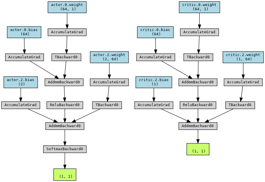
输出模型图片：

安装 torchsummary 包：

pip install torchsummary

代码：

from torchsummary import summary

device = torch.device("cuda:0" if torch.cuda.is_available() else "cpu")
print(device)
model = model.to(device)
summary(model, input_size=(state_dim,))

#查看模型参数
print("查看模型参数：")
for name, param in model.named_parameters():
    print(f"Layer: {name} | Size: {param.size()} | Values: {param[:2]}...")

输出：

cuda:0
—————————————————————-
        Layer (type)               Output Shape         Param #
================================================================
            Linear-1                   [-1, 64]             128
              ReLU-2                   [-1, 64]               0
            Linear-3                    [-1, 2]             130
           Softmax-4                    [-1, 2]               0
            Linear-5                   [-1, 64]             128
              ReLU-6                   [-1, 64]               0
            Linear-7                    [-1, 1]              65
================================================================
Total params: 451
Trainable params: 451
Non-trainable params: 0
—————————————————————-
Input size (MB): 0.00
Forward/backward pass size (MB): 0.00
Params size (MB): 0.00
Estimated Total Size (MB): 0.00
—————————————————————-
查看模型参数：
Layer: actor.0.weight | Size: torch.Size([64, 1]) | Values: tensor([[ 0.7747],
        [-0.0440]], device='cuda:0', grad_fn=<SliceBackward0>)…
Layer: actor.0.bias | Size: torch.Size([64]) | Values: tensor([ 0.5995, -0.2155], device='cuda:0', grad_fn=<SliceBackward0>)…
Layer: actor.2.weight | Size: torch.Size([2, 64]) | Values: tensor([[ 0.0373,  0.0851,  0.1000,  0.1060,  0.0387,  0.0479,  0.0127,  0.0696,
          0.0388,  0.0033,  0.1173, -0.1195, -0.0830,  0.0186,  0.0063, -0.0863,
         -0.0353,  0.0782, -0.0558,  0.0011, -0.0533,  0.1241,  0.0120, -0.0906,
         -0.0551, -0.0673, -0.1070,  0.0402, -0.0662,  0.0596, -0.0811,  0.0457,
          0.0349,  0.0564, -0.0155, -0.0404,  0.0843, -0.0978,  0.0459,  0.1097,
         -0.0858,  0.0736, -0.0067, -0.0756, -0.0363, -0.0525, -0.0426, -0.1087,
         -0.0611,  0.0420, -0.1038,  0.0402,  0.0065, -0.1217, -0.0467,  0.0383,
         -0.0217,  0.0283,  0.0800,  0.0228,  0.0415, -0.0473, -0.0199, -0.0436],
        [-0.1118, -0.0806, -0.0700, -0.0224,  0.0335, -0.0087,  0.0265, -0.1196,
         -0.0907, -0.0360,  0.0621, -0.0471, -0.0939, -0.0912, -0.1061,  0.1051,
         -0.0592, -0.0757,  0.0758, -0.1082, -0.0317,  0.1208, -0.0279, -0.0693,
          0.0920, -0.0318, -0.0476,  0.0236, -0.0761,  0.0591,  0.0862, -0.0712,
          0.0156, -0.1073,  0.1133,  0.0039, -0.0191,  0.0605, -0.0686, -0.1202,
          0.0962,  0.0581,  0.1145,  0.0741, -0.0993, -0.0987,  0.0939,  0.1006,
          0.0773, -0.0756, -0.1096,  0.0156, -0.0599,  0.0857,  0.1005, -0.0618,
          0.0474,  0.0066, -0.0531, -0.0479,  0.1136,  0.0356,  0.1169, -0.0023]],
       device='cuda:0', grad_fn=<SliceBackward0>)…
Layer: actor.2.bias | Size: torch.Size([2]) | Values: tensor([-0.0039,  0.0937], device='cuda:0', grad_fn=<SliceBackward0>)…
Layer: critic.0.weight | Size: torch.Size([64, 1]) | Values: tensor([[0.5799],
        [0.0473]], device='cuda:0', grad_fn=<SliceBackward0>)…
Layer: critic.0.bias | Size: torch.Size([64]) | Values: tensor([ 0.6507, -0.6974], device='cuda:0', grad_fn=<SliceBackward0>)…
Layer: critic.2.weight | Size: torch.Size([1, 64]) | Values: tensor([[ 0.0738, -0.0370, -0.1010, -0.0333, -0.0595, -0.0172,  0.0928,  0.0815,
          0.1221, -0.0842,  0.0511,  0.0452, -0.0386, -0.0503, -0.0964,  0.0370,
         -0.0341, -0.0693, -0.0845,  0.0424, -0.0491, -0.0439, -0.0443,  0.0203,
          0.0960, -0.1178, -0.0836, -0.0144, -0.0576, -0.0851,  0.0461,  0.1160,
          0.0120,  0.1180,  0.0255,  0.1047, -0.0398,  0.0786,  0.1143,  0.0806,
          0.1125,  0.0267,  0.0534, -0.0318,  0.1125, -0.0727,  0.1169,  0.0120,
         -0.0178, -0.0845,  0.0069,  0.0194,  0.1188,  0.0481,  0.1077, -0.0840,
          0.1013,  0.0586, -0.0857, -0.0974, -0.0630,  0.0359, -0.0080, -0.0926]],
       device='cuda:0', grad_fn=<SliceBackward0>)…
Layer: critic.2.bias | Size: torch.Size([1]) | Values: tensor([0.0621], device='cuda:0', grad_fn=<SliceBackward0>)…

到此这篇关于3种Python查看神经网络结构的方法小结的文章就介绍到这了,更多相关Python查看神经网络结构内容请搜索风君子博客以前的文章或继续浏览下面的相关文章希望大家以后多多支持风君子博客！

您可能感兴趣的文章:

• Python基于numpy灵活定义神经网络结构的方法
• Python调用graphviz绘制结构化图形网络示例
• python目标检测yolo1 yolo2 yolo3和SSD网络结构对比